Flow physics project
Project work: Monday, May 29, 13.00-17.00; Tuesday, May 30, 08.00-12.00 and 13.00-17.00; Wednesday, May 31, 13.00-17.00 in the group rooms Building 349, Ground floor
Project presentation preparation is Thursday from 8:00-12:00, and the presentations are from 13:00-17:00.
Purpose
The purpose of this project is to get familiar with the Womersley-Evans model for reconstruction of velocity profiles in different places in the human circulatory system. The students will have to generate their own flow data in specific simulated in vivo cases. The data for the project is simulated RF-data generated using Field II and the project builds on top of the exercise on velocity estimation.
Preparation
- Read chapter 3 in JAJ's book.
- Study the lecture slides from flow physics.
Methods
Data:
- Use the simulated RF data for flow in the femoral and carotid artery respectively to obtain the mean spatial velocity profile as a function of time.
- Data are located in the Dropbox folder under the assignment regarding flow physics.
The simulation parameters for the femoral artery are:
| Transducer: |
3 MHz, linear array probe with 64 elements |
| Pulse repetition frequency: |
15 kHz |
| Angle between flow and beam: |
70 degrees |
| Ultrasound pulse: |
4 cycles at 3 MHz |
| Sampling frequency: |
100 MHz |
| Resolution: |
16 bits samples |
| Position of vessel center: |
35 mm from transducer surface |
| Vessel radius: |
4.2 mm |
| Depth of first sample point: |
26.6 mm from transducer surface |
| Depth of last sample point: |
47.6 mm from transducer surface |
The file is called ''combined_data_femoralis_70_deg.mat'' and the Matlab variable ''data'' contains the RF data. One column contains the received RF signal for one pulse emission.
The file called ''parameters.mat'' holds the various variables used in the simulation.
Use the method you developed in the exercise on velocity estimation to obtain the mean spatial velocity as a function of time. This mean spatial velocity profile is the foundation for the reconstruction of the full velocity field as a function of time and space.
The simulation parameters for the carotid artery are:
| Transducer: |
5 MHz, linear array probe with 64 elements |
| Pulse repetition frequency: |
15 kHz |
| Angle between flow and beam: |
70 degrees |
| Ultrasound pulse: |
4 cycles at 5 MHz |
| Sampling frequency: |
100 MHz |
| Resolution: |
16 bits samples |
| Position of vessel center: |
25 mm from transducer surface |
| Vessel radius: |
3.0 mm |
| Depth of first sample point: |
19.0 mm from transducer surface |
| Depth of last sample point: |
34.0 mm from transducer surface |
The file is called ''combined_data_carotis_70_deg.mat'' and the Matlab variable ''data'' contains the RF data. One column contains the received RF signal for one pulse emission.
The file called ''parameters.mat'' holds the various variables used in the simulation.
Reconstruct the mean spatial velocity in the same way as you do for the femoral artery.
Data processing:
- For the femoral artery, plot the mean spatial velocity as a function of time. How long is the cardiac cycle?
- Use the mean spatial velocity profile to reconstruct the full velocity profile as a function of both time and space using the Womersley-Evans model. Plot the result as a function of time and space. Try out different visualisations.
- Calculate the volume flow rate assuming that the vessel has a circular symmetric cross-section. Plot the volume flow rate as a function of time.
- Repeat the data processing for the common carotid artery.
- Compare and discuss your results. Is the flow laminar or turbulent? Why do we not see fully-developed flow in these vessels?
Expected results:
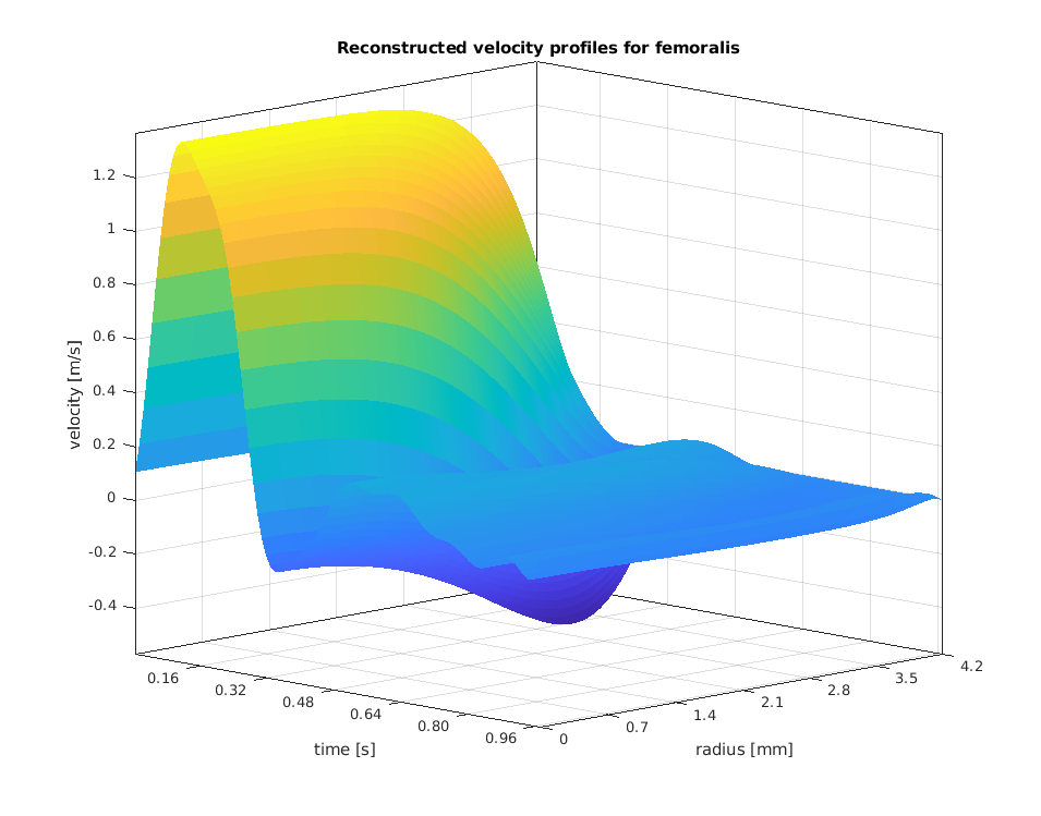
Pulsatile flow, femoral artery
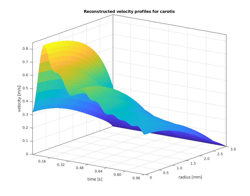
Pulsatile flow, carotid artery
Example code for the Womersley-Evans model
 %% ======= CALCULATION OF PSI ======= %%

 % The equations for reconstructing the velocity profiles are given in
 % Estimation of Blood Velocities Using Ultrasound: A Signal Processing
 % Approach, 2nd Edition on pages 55-58.

 % Psi is given in eq. (3.27b)

 psi = 0;
 % J is the number of harmonics in the spectral decomposition of the spatial mean velocity
 for p = 1:J
    omega = p*omega_0;    % harmonic angular frequency
    tau_p = sqrt(-1)^(3/2)*R*sqrt(omega*rho/mu);
    index = 1;
    % calculating psi for each radial position
    for r_rel = 0:deltaR:0.99
        Be = tau_p*besselj(0,tau_p); % first term in the nominator and denominator
        psi(index,p) = (Be - tau_p*besselj(0,r_rel*tau_p))/(Be - 2*besselj(1,tau_p));
        index = index + 1;
    end
 end
Parameters needed for the Womersley-Evans model implementation:
| '''Parameter''' |
'''Value''' |
'''Description''' |
| R |
4.2 or 3.0 mm |
Vessel radius, given in ''parameters.mat'' |
| Ï |
1.060 kg/m3 |
Blood density |
| μ |
0.004 Pa·s |
Blood viscosity |
| bpm |
62 |
Heart beats perminute |
T |
0.968 s |
Length of the cardiac cycle |
| J |
8-10 |
Number of harmonics in the spectral decomposition |
| F |
1/T |
Harmonic frequency |
| Ï |
2 Ï F |
Angular frequency |
| v0 |
- m/s |
Peak velocity of the fully-developed profile, given in ''parameters.mat'' |
| rsam |
20 |
Number of radial samples in the reconstruction |
| tsam |
40 |
Number of temporal samples in the reconstruction |
Papers and reading material:
- Brandt, A. H., Hansen, K. L., Ewertsen, C., Holbek, S., Olesen, J. B., Moshavegh, R., Thomsen, C., Jensen, J. A., & Nielsen, M. B. (2018). A Comparison Study of Vector Velocity, Spectral Doppler and Magnetic Resonance of Blood Flow in the Common Carotid Artery. Ultrasound in Medicine and Biology, 44(8), 1751-1761
- Jensen, J., Villagómez Hoyos, C. A., Traberg, M. S., Olesen, J. B., Tomov, B. G., Moshavegh, R., Holbek, S., Stuart, M. B., Ewertsen, C., Hansen, K. L., Thomsen, C. E., Nielsen, M. B., & Jensen, J. A. (2018). Accuracy and Precision of a Plane Wave Vector Flow Imaging Method in the Healthy Carotid Artery. Ultrasound in Medicine and Biology, 44(8), 1727-1741
- Holbek, S., Hansen, K. L., Bouzari, H., Ewertsen, C., Stuart, M. B., Thomsen, C. E., Nielsen, M. B., & Jensen, J. A. (2017). Common Carotid Artery Flow Measured by 3-D Ultrasonic Vector Flow Imaging and Validated with Magnetic Resonance Imaging. Ultrasound in Medicine and Biology, 43(10), 2213-2220
Dissemination:
Make a 10 minutes presentation of your project, which will be discussed on Thursday, June 1 from 13:00. There is 15 minutes available for each project group.
|

 Print Version