Row-column beamformation

Friday, May 29, 10.00-12.00 in the group rooms Building 349, Ground floor /

Purpose:

The purpose of this exercise is to beamform ultrasound RF data acquired with a row-column (RC) probe using the conventional beamformation algorithm developed by M. F. Rasmussen, et al. data.

Preparation:

Read lecture slides and the journal paper by Rasmussen et al. found in the row-column beamformation section in the course notes. Finish the beamformation exercise from day one.

Exercise:

1. Load exercise data into MATLAB.

load('exercise05_sim.mat') % simulated data
% load('exercise05.mat') % measured data (carotid artery phantom)

This mat-file contains the following parameters:



Variable name	Content	Unit
data	Complex matched filtered RF data for each emission - Size: [#samples, #elements, #emissions]	$\backslash sim$
fs	Sampling frequency (31.25 MHz)	Hz
t_start	Start time for RF data.	s
c	Speed of sound in the medium	m/s
f0	Pulse's center frequency	Hz
ele_pos	Center (x,y,z)-positions of the receiving elements (*)	m
src_pos	Center (x,y,z)-positions of the emission line source (*)	m

(*) The receiving elements are, in this course, assumed to be the column elements, and the transmitting elements are assumed to be the row elements.


2. Use the built-in function "plot3" to visualize the center positions of the emission source and the receiving elements. In which direction does the emission source change and in which direction does the element position change?


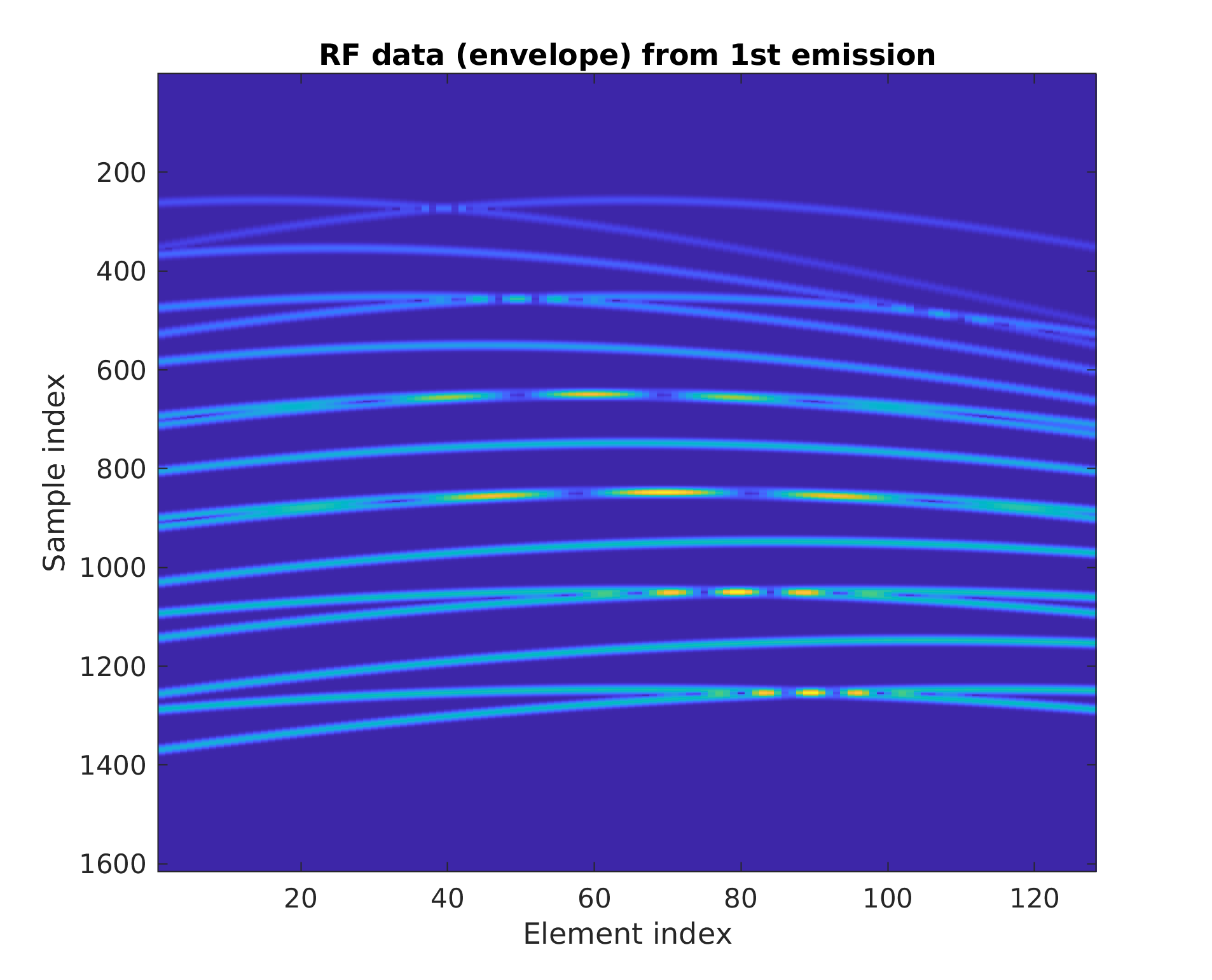
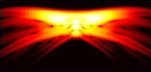
3. Make an image of the RF data from the first emission. It should look similar to the image shown below. Convert the "Sample index" axis into time. Hint: use variables "t_start" and "fs".




4. Use the time of flight (ToF) equation (see equation below) to calculate the ToF-profile (i.e., the ToF to each element) for a single image point located at $(x,y,z)\; =\; (0,0,27.5)$ mm. Plot the ToF-profile on top of the RF data image. If calculated correctly, the ToF-profile should align with one of the curves in the RF data image.



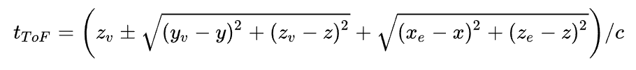
Emission source's (y,z)-position: (y_v,z_v)
Receiving element's (x,z)-position: (x_e,z_e)
Note that the +/- sign is + if z>z_v_v and - otherwise.


5. Interpolate the complex RF-data along the ToF profile and sum the interpolated values. Combining this output for each emission yields the beamformed image point at (x,y,z) = (0,0,27.5) mm. Hint: use interp1(...,'spline',0)


6. Beamform an xz-plane (y=0 mm) and a yz-plane (x=0 mm). The planes' range should be z in [10, 45] mm and x and y in [-12, 12] mm. The sampling interval in x, y, and z should be lambda/2 = (c/f_0)/2. The final output should look similar to the images below(*).



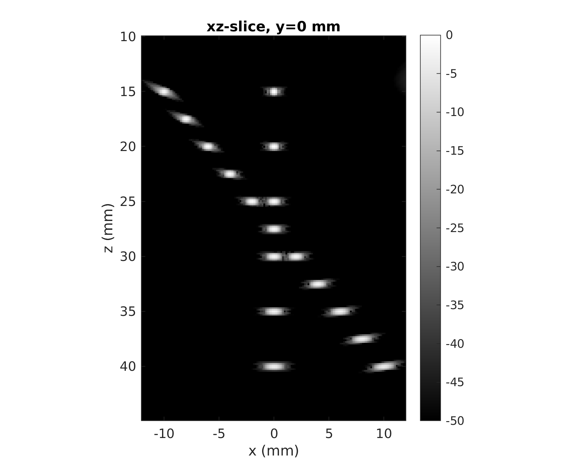
B-mode xz-slice



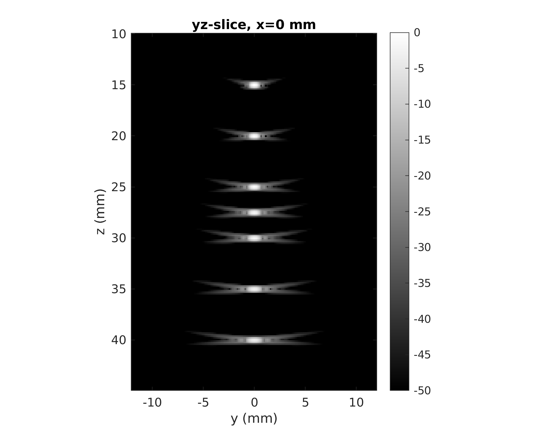
B-mode yz-slice

(*) Side-lobe levels might vary do to difference in apodization.